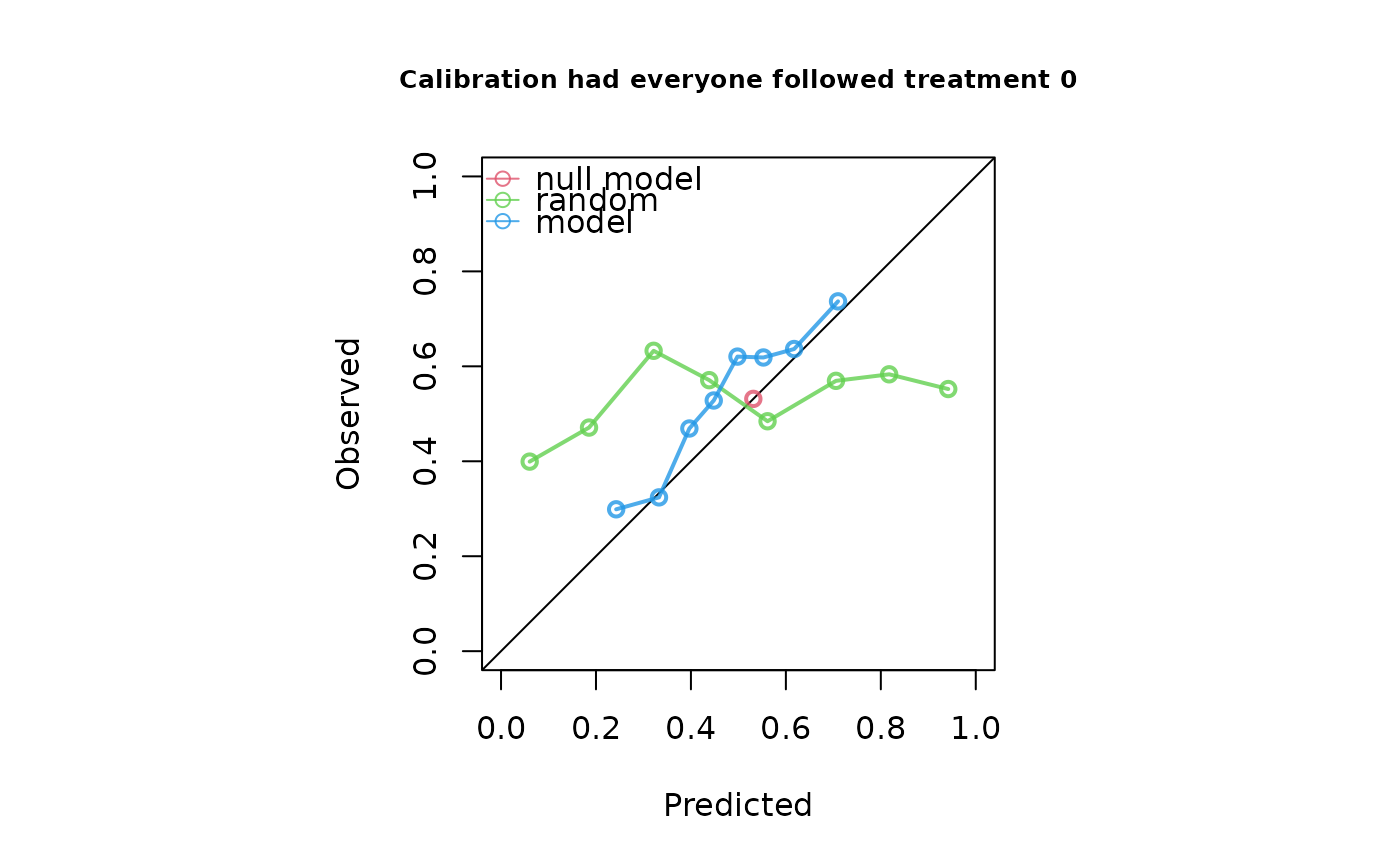
Produces a calibration plot comparing predicted and observed outcomes under the intervention of interest.
Arguments
- x
The `ip_score` object returned by
ip_score- xlim
The x limits of the plot, c(x1, x2)
- ylim
The y limits of the plot, c(y1, y2)
- pty
A character specifying the type of plot region to be used; "s" generates a square plotting region and "m" generates the maximal plotting region.
- asp
The y/x aspect ratio
- main
Character string giving the main title of the plot.
- xlab
Character string specifying the x-axis label.
- ylab
Character string specifying the y-axis label.
- cex.main
Numeric value controlling the size of the main title.
- legend
Keyword denoting the positioning of the legend. Can be "bottomright", "bottom", "bottomleft", "left", "topleft", "top", "topright", "right" and "center", or alternatively, "none" to hide the legend.
- ...
Currently ignored.
Details
Subjects are grouped into subgroups according to percentiles of the estimated risks. For each subgroup, the x-coordinate is the mean estimated risk of the subgroup. The y-coordinate is the inverse-probability-weighted proportion of 'observed' events.
The observed and predicted calibration subgroup coordinates are computed by the
ip_score function and are stored
in `x$score$calplot`, where `x` is the `ip_score` object. These raw values
can be used to create custom calibration plots when additional control is
needed.
If ip_score was run with
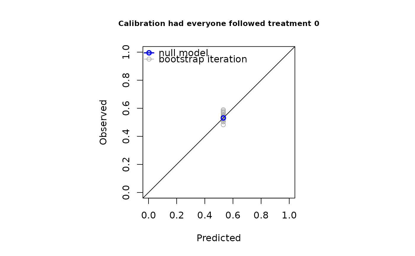
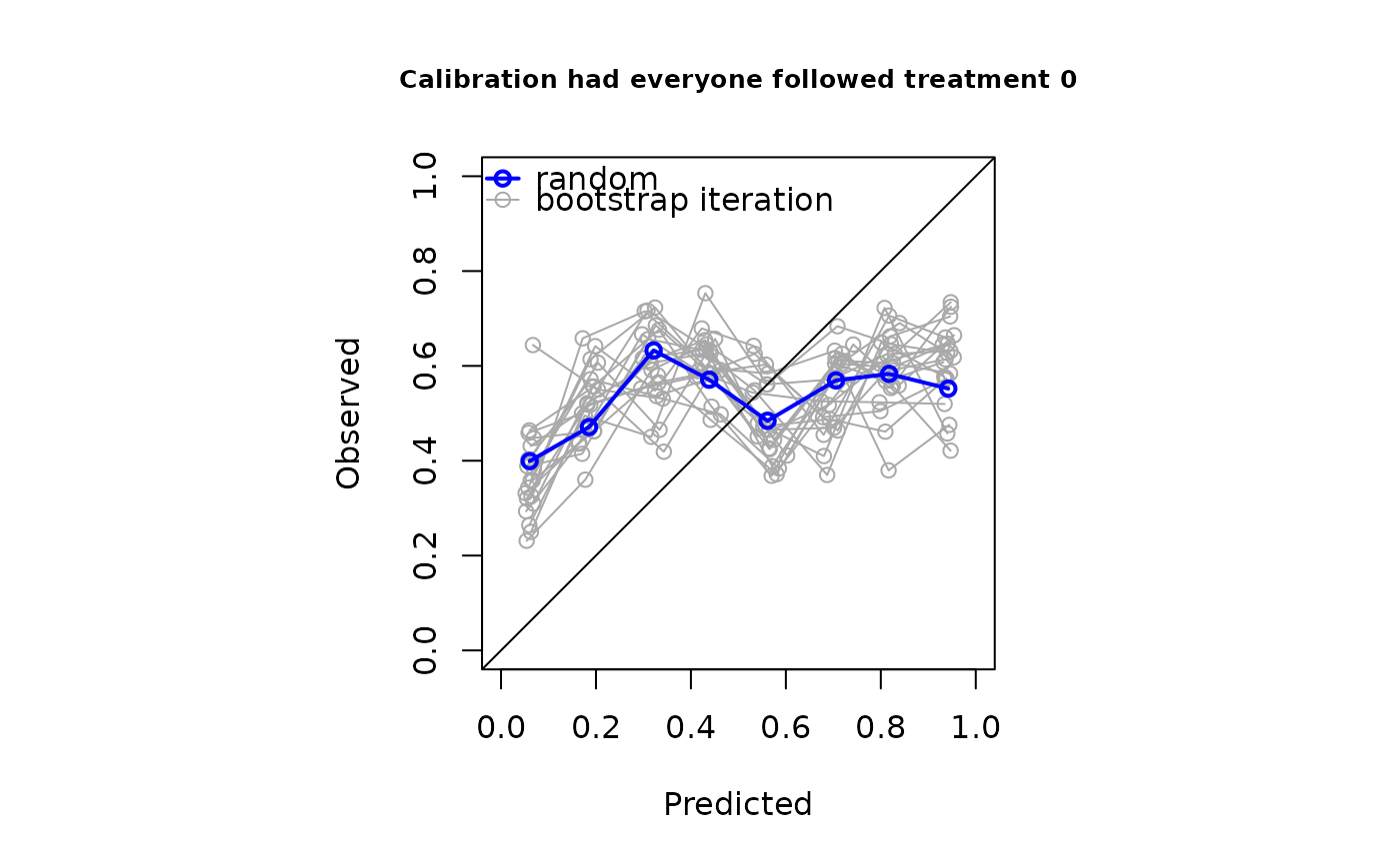
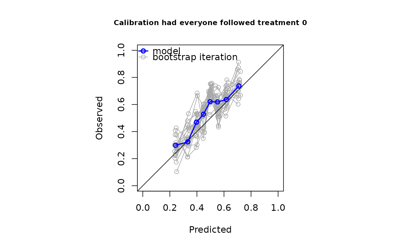
bootstrap resampling (`bootstrap > 0`), additional panels are produced for
every evaluated model showing the calibration curves from all bootstrap
replicate in grey.
This method is available only when "calplot" was included in the `metrics`
argument of ip_score.
Examples
n <- 1000

data <- data.frame(L = rnorm(n), P = rnorm(n))
data$A <- rbinom(n, 1, plogis(data$L))
data$Y <- rbinom(n, 1, plogis(0.1 + 0.5*data$L + 0.7*data$P - 2*data$A))

random <- runif(n, 0, 1)
model <- glm(Y ~ A + P, data = data, family = "binomial")

score <- ip_score(
  object = list(random, model),
  data = data,
  outcome = Y,
  treatment_formula = A ~ L,
  treatment_of_interest = 0,
  bootstrap = 20,
  bootstrap_progress = FALSE,
  metrics = "calplot"
)

plot(score)