1 The special nature of survival data

This file contains R code for the analyses in Chapter 1 of the book Dynamic Prediction in Clinical Survival Analysis (CRC Chapman & Hall) by Hans C. van Houwelingen and Hein Putter

R code written by Hein Putter (H.Putter@lumc.nl for comments/questions) The dynpred package is available from CRAN

Consistency with the book has been checked with - R version 2.14.0 - survival version 2.36-10 - dynpred version 0.1.1

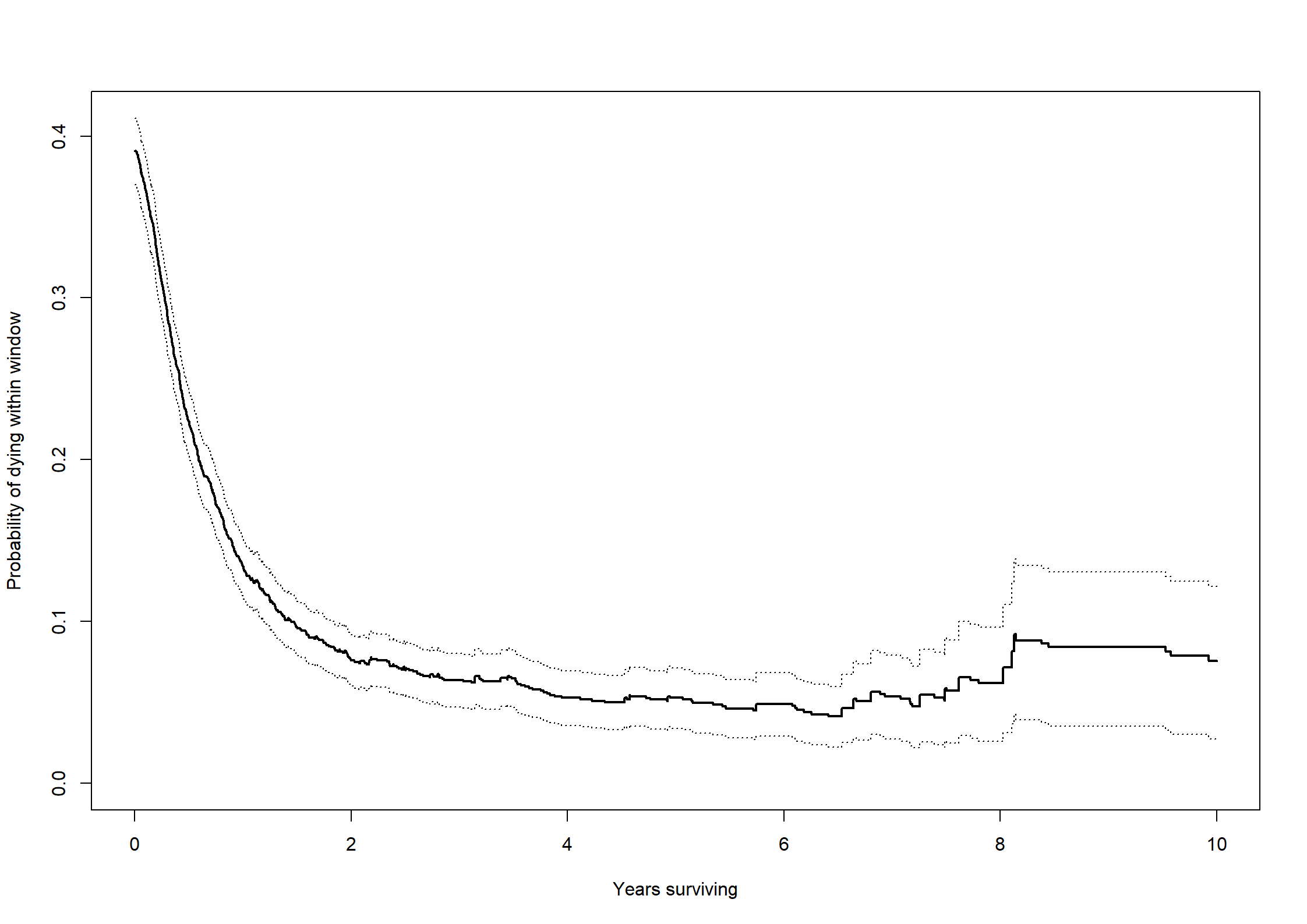
Figure 1.1: Probability of death or relapse within the next 5 years in Data Set 6 (ALL)

Code

require(dynpred)
data(ALL)

year <- 365.25

# Define relapse-free survival as the earliest of relapse and death
# Time to relapse (rel) and time to death (srv) are in days
# RFS will be in years
ALL$rfs <- pmin(ALL$rel,ALL$srv)/year
ALL$rfs.s <- pmax(ALL$rel.s,ALL$srv.s)

# The function Fwindow (from dynpred) is used; it takes a survfit
# object
c0 <- coxph(Surv(rfs,rfs.s) ~ 1, data=ALL, method="breslow")
sf0 <- survfit(c0)
Fw <- Fwindow(sf0,5)

# Plot first 10 years
Fw <- Fw[Fw$time<=10,]
plot(Fw$time,Fw$Fw,type="s",ylim=c(0,max(Fw$up)),xlab="Years surviving",ylab="Probability of dying within window",lwd=2)
lines(Fw$time,Fw$low,type="s",lty=3)
lines(Fw$time,Fw$up,type="s",lty=3)

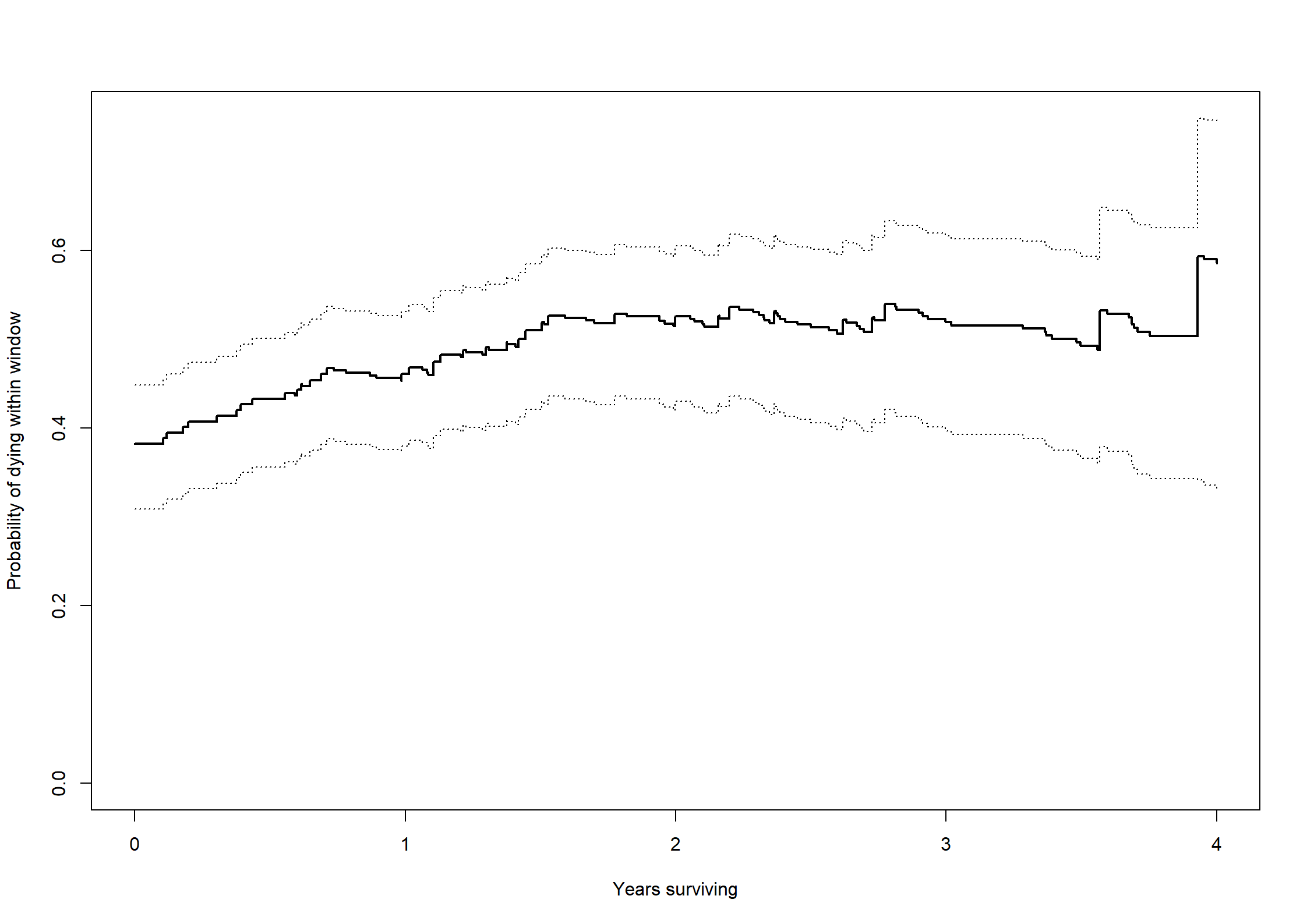
Figure 1.2: Probability of dying within the next 4 years in Data Set 2 (CML data)

Code

data(wbc1)

c0 <- coxph(Surv(tyears, d) ~ 1, data = wbc1, method="breslow")
sf0 <- survfit(c0)
Fw <- Fwindow(sf0,4)

# Plot first 4 years
Fw <- Fw[Fw$time<=4,]
plot(Fw$time,Fw$Fw,type="s",ylim=c(0,max(Fw$up)),xlab="Years surviving",ylab="Probability of dying within window",lwd=2)
lines(Fw$time,Fw$low,type="s",lty=3)
lines(Fw$time,Fw$up,type="s",lty=3)

Figure 1.3 (data unfortunately not available)

Code

library(foreign)

d1d2 <- read.spss("D1d2.sav",to.data.frame=TRUE)
names(d1d2) <- casefold(names(d1d2))

d1d2 <- d1d2[d1d2$instud=="curative",]
d1d2 <- d1d2[,c(4,5,11,12,22,27,31,34,38,46:49,51,59,71,72,86,88,90,91)]
d1d2$patid <- row.names(d1d2)

d1d2$status <- as.numeric(d1d2$status)-2

# Separately for D1 vs D2-dissection
c1 <- coxph(Surv(survyo, status) ~ 1, data=d1d2, subset=(randgr=="D1"), method="breslow")
sf1 <- survfit(c1)
Fw1 <- Fwindow(sf1,4,variance=FALSE)
c2 <- coxph(Surv(survyo, status) ~ 1, data=d1d2, subset=(randgr=="D2"), method="breslow")
sf2 <- survfit(c2)
Fw2 <- Fwindow(sf2,4,variance=FALSE)

# Plot first 6 years
Fw1 <- Fw1[Fw1$time<=6,]
Fw2 <- Fw2[Fw2$time<=6,]

plot(Fw1$time,Fw1$Fw,type="s",ylim=c(0,max(c(Fw1$Fw,Fw2$Fw))),xlab="Years surviving",ylab="Probability of dying within window",lwd=2)
lines(Fw2$time,Fw2$Fw,type="s",lwd=2,col=8)
legend("topright",c("D1","D2"),lwd=2,col=c(1,8),bty="n")