5  Mechanisms explaining violation of the Cox model

This file contains R code for the analyses in Chapter 5 of the book Dynamic Prediction in Clinical Survival Analysis (CRC Chapman & Hall) by Hans C. van Houwelingen and Hein Putter

R code written by Hein Putter (H.Putter@lumc.nl for comments/questions) The dynpred package is available from CRAN

Consistency with the book has been checked with - R version 2.14.0 - survival version 2.36-10 - dynpred version 0.1.1

Code

###############################################################################
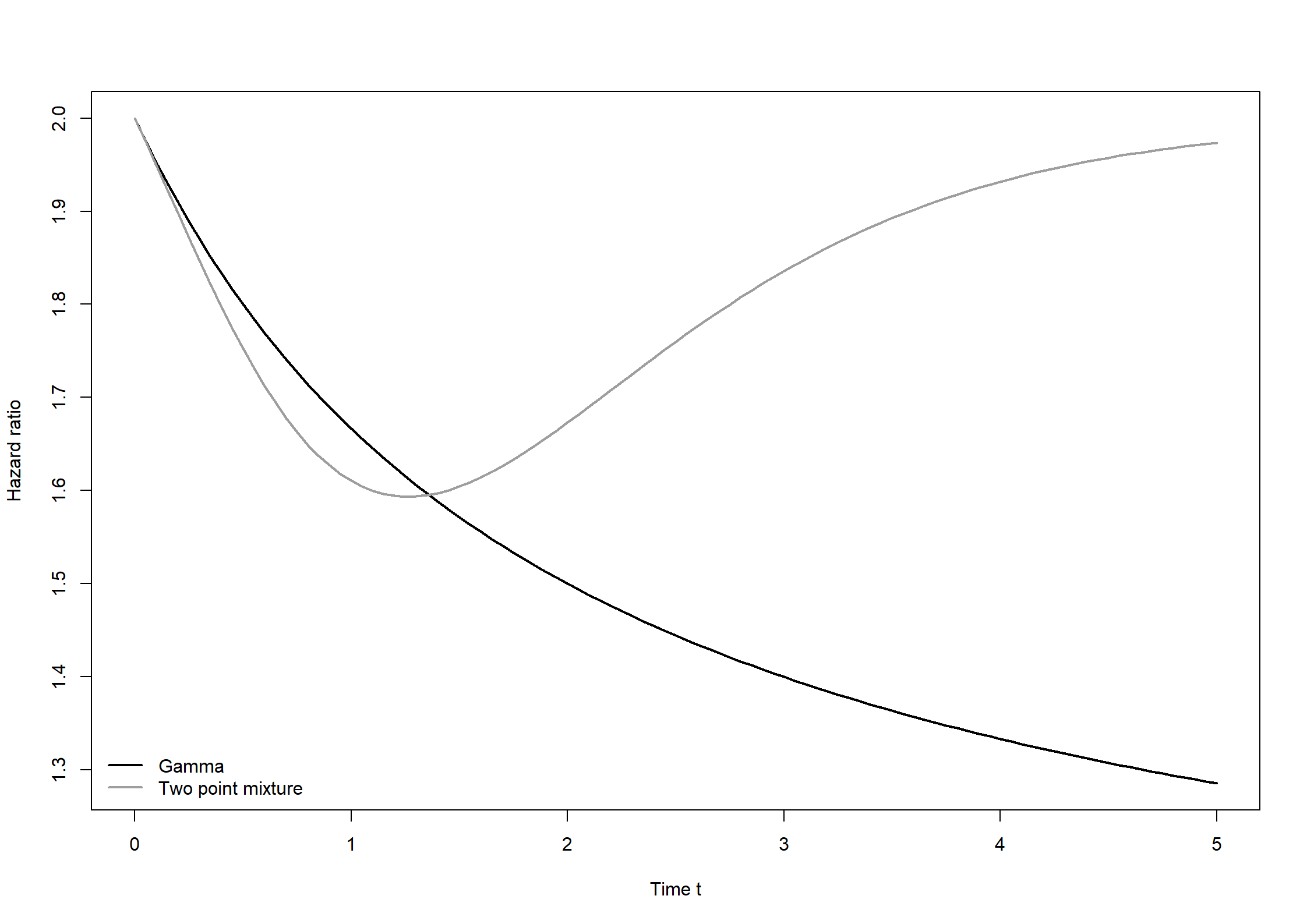
### Figure 5.1: Hazard ratio for simple model for gamma and mixture
### frailty distribution
###############################################################################

HR <- 2
h0 <- function(t) 1
H0 <- function(t) t
h1 <- function(t) HR*h0(t)
H1 <- function(t) HR*H0(t)

# Gamma frailty (abbreviation g)
th <- 4
h0g <- function(t) (th*h0(t))/(th + H0(t))
h1g <- function(t) (th*h1(t))/(th + H1(t))
# Two-point mixture frailty (abbreviation m)
p <- 0.5; xi0 <- 0.5; xi1 <- 1.5
EZ0 <- function(t) ((1-p)*xi0+p*xi1*exp(-(xi1-xi0)*H0(t)))/((1-p)+p*exp(-(xi1-xi0)*H0(t)))
EZ1 <- function(t) ((1-p)*xi0+p*xi1*exp(-(xi1-xi0)*H1(t)))/((1-p)+p*exp(-(xi1-xi0)*H1(t)))
h0m <- function(t) EZ0(t)*h0(t)
h1m <- function(t) EZ1(t)*h1(t)

tseq <- seq(0,5,by=0.05)
HRgseq <- h1g(tseq)/h0g(tseq)
HRmseq <- h1m(tseq)/h0m(tseq)

plot(tseq,HRgseq,type="l",lwd=2,xlab="Time t",ylab="Hazard ratio")
lines(tseq,HRmseq,type="l",lwd=2,col=8)
legend("bottomleft",c("Gamma","Two point mixture"),lwd=2,col=c(1,8),bty="n")

Code

###############################################################################
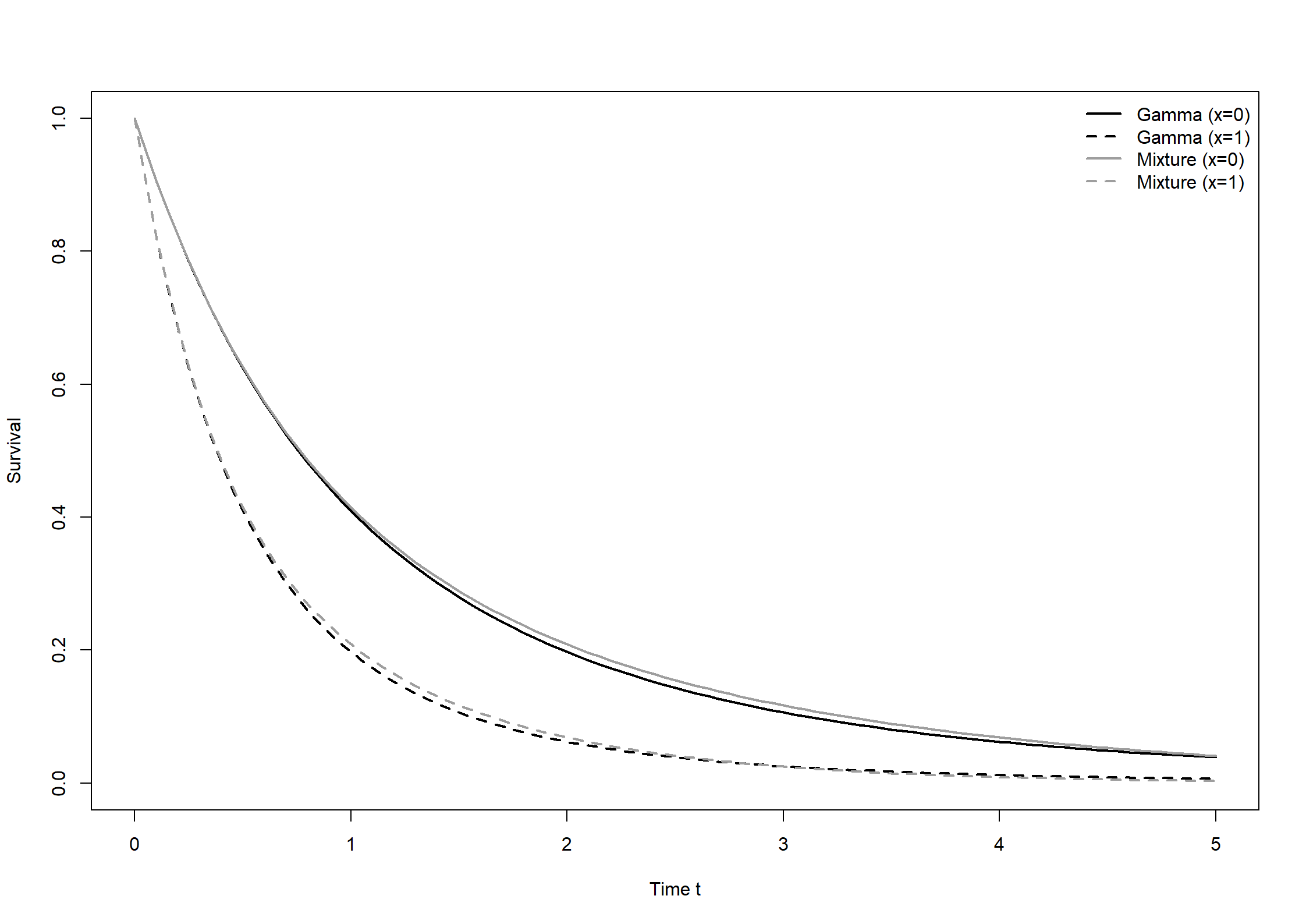
### Figure 5.2: Marginal survival in the two groups under the two models
###############################################################################

nseq <- length(tseq)
S0g <- S1g <- S0m <- S1m <- rep(NA,nseq)
for (j in 1:nseq) {
    S0g[j] <- integrate(h0g, 0, tseq[j])$value
    S1g[j] <- integrate(h1g, 0, tseq[j])$value
    S0m[j] <- integrate(h0m, 0, tseq[j])$value
    S1m[j] <- integrate(h1m, 0, tseq[j])$value
}

plot(tseq,exp(-S0g),type="l",lwd=2,ylim=c(0,1),xlab="Time t",ylab="Survival")
lines(tseq,exp(-S1g),type="l",lwd=2,lty=2)
lines(tseq,exp(-S0m),type="l",lwd=2,col=8)
lines(tseq,exp(-S1m),type="l",lwd=2,lty=2,col=8)
legend("topright",c("Gamma (x=0)","Gamma (x=1)","Mixture (x=0)","Mixture (x=1)"),lwd=2,col=c(1,1,8,8),lty=c(1,2,1,2),bty="n")

Code

###############################################################################
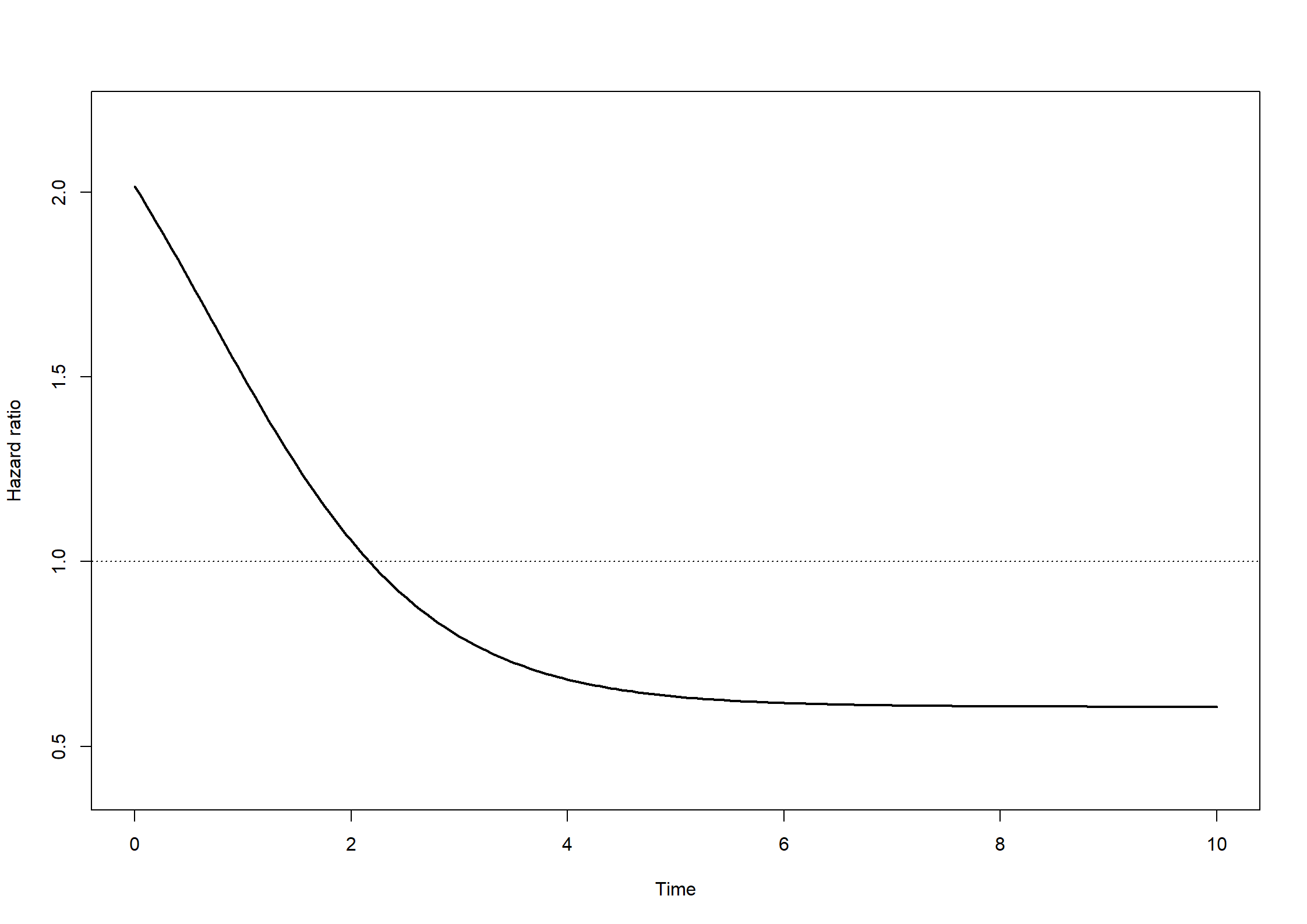
### Figure 5.3: Hazard ratio for ?imitation? of Data Set 5
###############################################################################

HR1 <- exp(1)
HR2 <- exp(-0.5)
h10 <- function(t) 0.2*exp(-t)
h20 <- function(t) 0.1
h0 <- function(t) h10(t) + h20(t)
h11 <- function(t) h10(t)*HR1
h21 <- function(t) h20(t)*HR2
h1 <- function(t) h11(t) + h21(t)
HR <- function(t) h1(t)/h0(t)
tseq <- seq(0,10,by=0.05)
HRseq <- HR(tseq)

plot(tseq,HRseq,type="l",lwd=2,ylim=c(0.4,2.2),xlab="Time",ylab="Hazard ratio")
abline(h=1,lty=3)

Code

###############################################################################
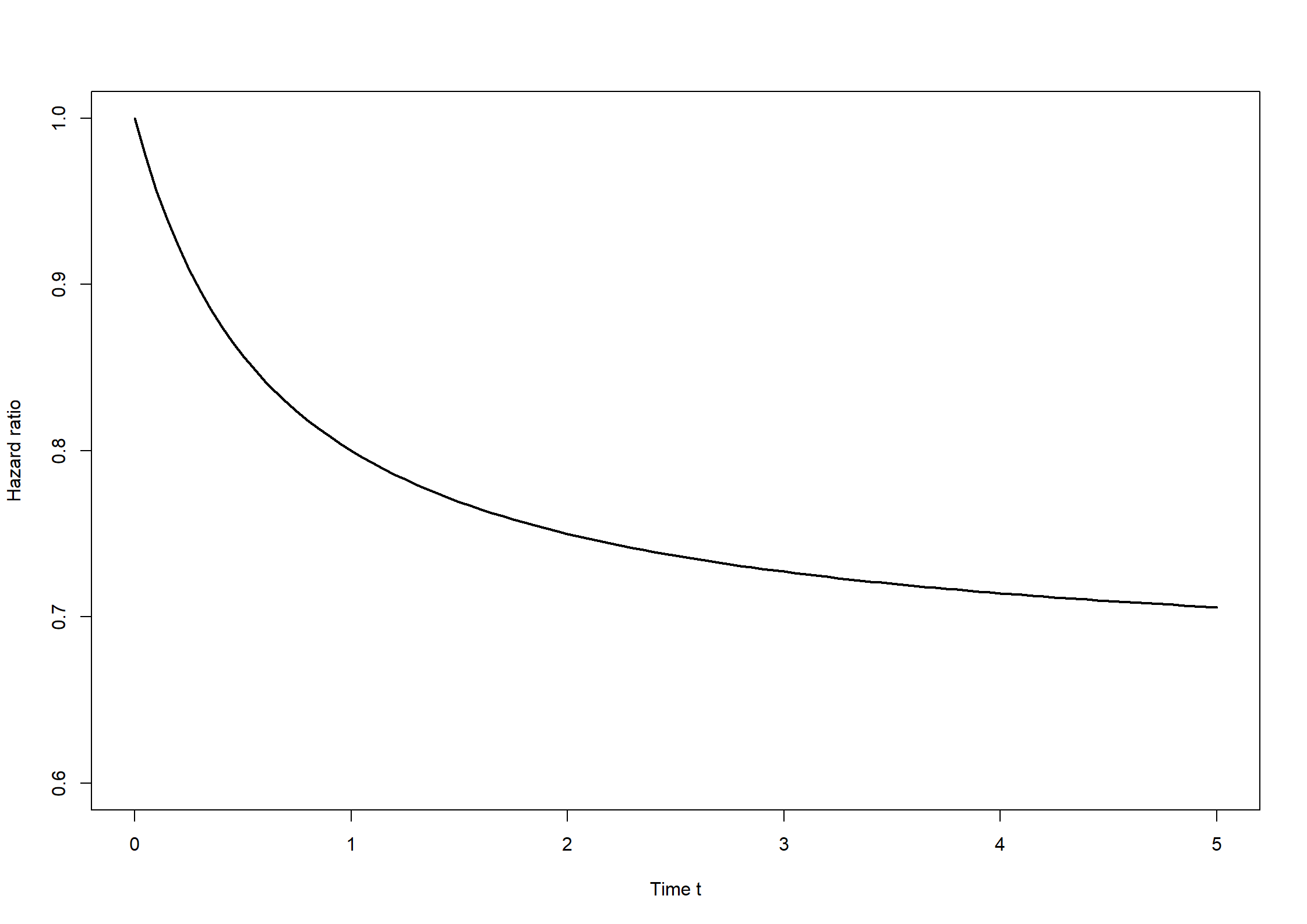
### Figure 5.4: Hazard ratio for the marginal cause-specific hazard of cause 1,
### for the shared gamma frailty model with variance 0.5
###############################################################################

HR1 <- 1
HR2 <- 2
th <- 0.5
h10 <- function(t) 1
h20 <- function(t) 1
H10 <- function(t) t
H20 <- function(t) t

h10g <- function(t) h10(t)/(1 + th*(H10(t)+H20(t)))
h11g <- function(t) (h10(t)*HR1)/(1 + th*(HR1*H10(t)+HR2*H20(t)))
tseq <- seq(0,5,by=0.05)
HRgseq <- h11g(tseq)/h10g(tseq)

plot(tseq,HRgseq,type="l",lwd=2,ylim=c(0.6,1),xlab="Time t",ylab="Hazard ratio")
lines(tseq,HRmseq,type="l",lwd=2,col=8)